ZKsync Prover Optimizations

11 Dec, 2024

"Algorithmics is easy, don't do anything dumb, don't do anything twice, you're good to go." -- first heard from Errichto, unknown original author

TL;DR; Optimizations for ZKsync provers:

1. Reduced the compute cost. Depending on chain's TPS, this can range between 20x (low TPS chains -- TPS <= 0.1) to 5x (higher TPS chains -- TPS >= 2).
2. Reduced execution time. Additionally, there is a lever in place that has a spectrum between cheap & slow proving to expensive & fast proving.
3. Removed previous bottlenecks and improved scalability. No load tests have been done to identify the ceiling, but more than 5x TPS is possible.
4. Removed vendor lock-in (can run on various cloud compute providers¹)

Context

The proving process can be thought of as a task pipeline. The tasks form a Direct Acyclic Graph (DAG) that needs to be executed. It has a single "root" node and a single "leaf" node. The root of the tree is the batch information that has to be turned into circuit proofs to be proven & aggregated. The leaf node is the aggregated proof that ends up on on-chain. Nodes of DAG are not fungible. Nodes run different software, have different execution times & hardware requirements.

The following diagram show-cases the proving DAG².

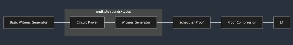
A technical description of what has been done on each component (that was optimised) follows.³

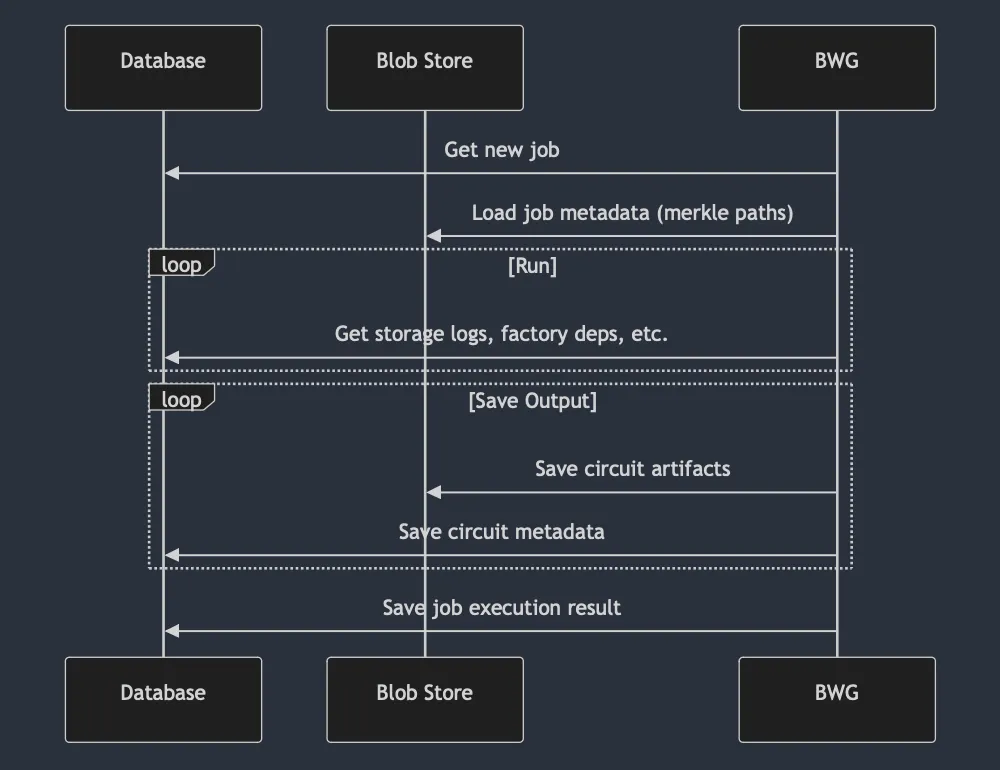
Basic Witness Generator

Basic Witness Generation is the process that kickstarts the proving workflow. It is responsible for computing the geometry of the batch (how many layers of circuit proofs will be necessary and of which types). Previous architecture:

Improvements

1. Remove database queries

The process keeps querying the database. This has 2 problems:

• execution flow is throttled by the round-trip to the database
• SQL databases can be unpredictable (table size & selection of index can result in wildly different response times -- there's no SLA)

All the data can be precomputed and loaded at runtime straight to memory. This solves both problems. It also enables full decoupling between proving and sequencer (no need to access sequencer database).

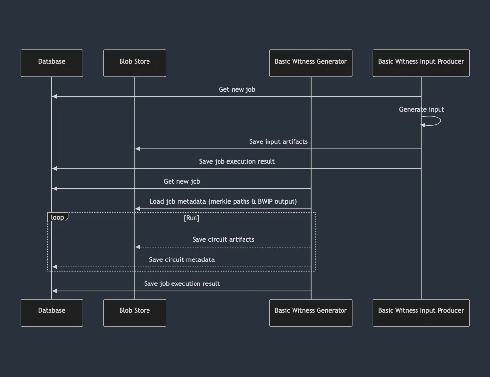
For implementation, Basic Witness Input Producer (BWIP) generates the needed data. All BWG inputs are packed together and sent at once via prover gateway (not pictured in the sequence diagram). BWG is 100% independent and can run without any external accesses from this point onwards.

2. Optimize processing logic

Initially, the batches were rather small (think < 1k circuits). Given Era's success, batches became large (~1 order of magnitude increase). Algorithms that previously worked ok (linear search over some hundred fields) became too slow. There are multiple instances where we tuned the process to work on bigger inputs by simply applying sensible algorithms.

3. Stream circuits

The processing collects all circuits in the run and then provides them all as output. An alternative is to provide circuits async as they are computed, rather than all at the end. This brings two main advantages:

• you can save circuits async whilst the processing is ongoing
• you can deallocate the circuit as soon as it's been persisted

Whilst it may not seem like much, this alone shaved ~10% of the execution time and reduced the memory footprint 5 times.

4. Reduce the size of transferred data

Not all data transferred back and forth between circuits is necessary. Some of it can be blanked out at runtime or simply exists for convenience within the witness generation process, but provides no benefit for proving. Stripping this information saves us costs on network transfer, storage & memory allocation/deallocation.

Results

Putting it all together:

Execution time decreased one order of magnitude⁴. Using less compute makes it cheap on a similar level of magnitude.

Note: All other witness generators benefit from reduced data size transferred across processes.

Future Improvements

• There is space to reduce even further the data transferred back and forth
• There is space for more parallelism in the design
• Better hardware can be used to take advantage of the type of processing done (mostly hashing)

Circuit Prover

Circuit Prover is the critical path for proving. It gets a circuit, prepares the information (vector generation) and then proves it (usually accelerated on GPUs). This component is the most expensive (~75% of cost) part of the proving infrastructure. Previous Circuit Proving architecture looks like this:

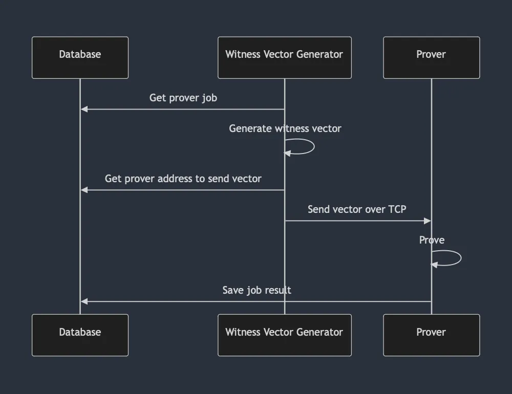
Note 1: Witness Vector Generator (WVG) & Prover ℗ are 2 processes running on different machines (expected to be in same Availability Zone).

Note 2: All circuits are grouped into "prover groups" -- this means X (usually <= 4) circuits belong to a single group and a prover is of a specific group type (therefore can prove only its group's X types of circuits)

Improvements

1. Make WVG single threaded

WVG runs across multiple threads. Moving it to single threaded setup lowers the overall CPU utilization.

2. Run WVG & P on the same machine

WVG are CPU heavy jobs, whilst P are GPU heavy. In the past, those were split as the GPU would be mostly idle waiting for CPU bound workload. Given machine pricing & availability, the sensible cost approach was simply split the workloads and have dedicated machines for each.

The changes in WVG from point 1 reduced the required number of cores per machine from ~55 to ~23. Such machines are available on different cloud vendors (and they are standard configuration, which keeps price down).

3. Get rid of prover groups

Prover groups are good for reusing GPU cache⁵ & having low memory utilization⁶.

The problem with specialization is that there can be provers running that have no work to do and are pending to shut down. Without work stealing (take proofs from other groups), the machines are bound to idle.

The alternative is to have a single type of prover that can prove all circuits. Post boojum, setup data size reduced from ~10GB to ~700MB (per circuit). A machine with all circuits would need ~40GB of RAM, instead of ~580GB previously. As with WVG changes, there are such machines at reasonable prices & availability that fulfil the requirements.

4. Run everything in parallel

As noted in the diagram, all processes are fully synchronous. One could get better utilization by loading and offloading data off the GPU in parallel, whilst the GPU is crunching through proving. This is relevant in prover context, because GPU proving is < 1s. If your loading & offloading is ~1s, you reduced your capacity by half (not accounting for P99 and tail latencies).

Note: Parallel running can be applied to all prover components, but circuit provers see the biggest improvement.

Results

The new pipeline looks as follows:

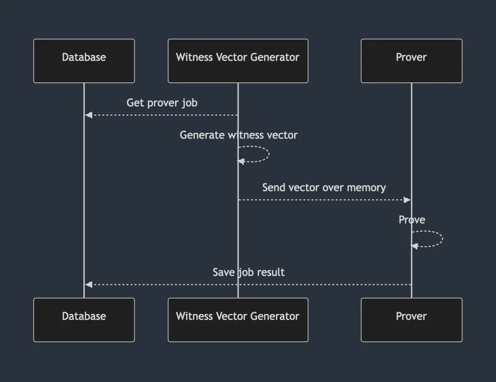
With:

• Proof generation reduced over P90 to <30s (from 1m:21s)
• All witness vector generator machines decomissioned in favor of utilizing CPUs that come alongside the GPU. This alone halves the cost.
• A low TPS chain would require an order of magnitude less GPUs (observed as 14x), whilst higher TPS chains would require ~5x less GPUs.
• Removing Witness Vector Generator & Prover separation makes proving pipeline cloud agnostic. Previously, GCP context was necessary to determine if 2 machines ran in the same Availability Zone.
• Scalability improved an order of magnitude. Previously, ~20 pods were necessary to cover what the new prover can. This meant ~20 connections to the database and polls. With new setup, only 3 are necessary and they are throttled by execution time.
• GPU availability is a bottleneck for current setup. Requiring less GPUs gives more breathing space during peak TPS.

Future Improvements

This implementation is v1. Running Circuit Provers in production provides more insight into how to fine-tune configuration to infrastructure (planned for the near future).

Proof Compression

Proof Compressor is the last component that takes the scheduler FRI proof and turns it into a PLONK proof.

Improvements

1. GPU accelerate proving generation

Proof compression has a proving part. Previous proving ran on CPUs. This was slow and time intensive. Moving it to GPU sped it up. Even though the GPU machine is more expensive, running it an order of magnitude less time makes the entire setup cheaper.

2. Rethink hashing

It has been identified that choice of hashing function slowed down the compression. Replacing hashing reduced the run-time further..

Results

Compression moved from ~30 minutes execution time to < 3 minutes.

Future Improvements

• PLONK setup is expensive to verify on L1. A different setup would enable us to lower verification further (cost reduction on-chain)

Prover Autoscaler

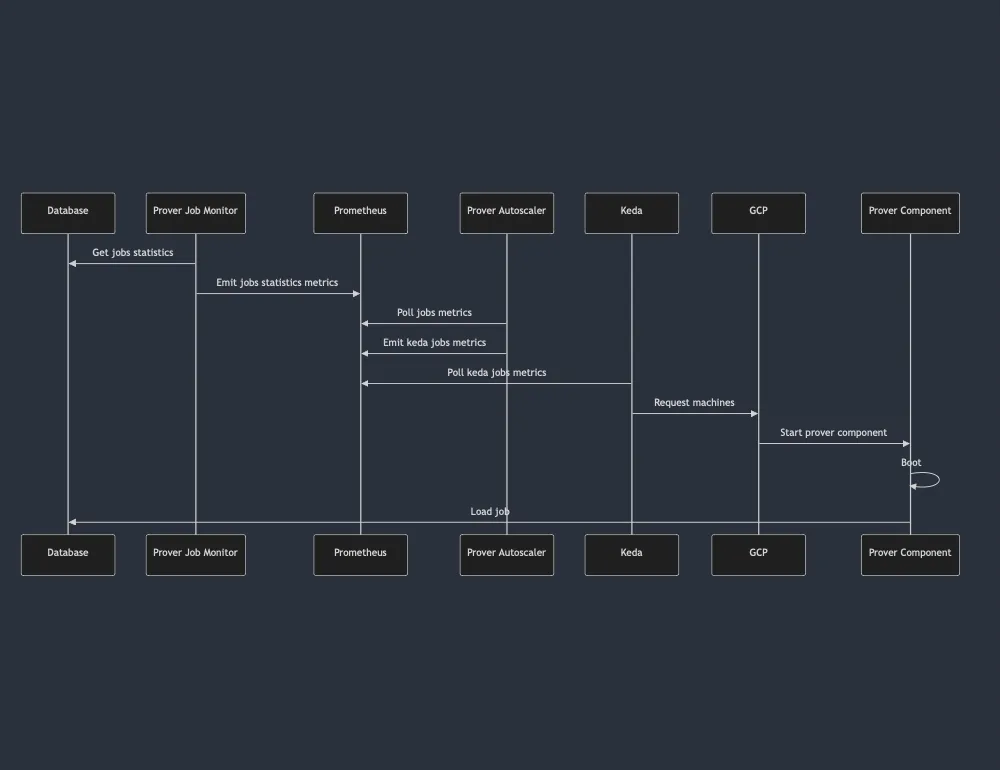
Proving is parallelizable across multiple machines & requires multiple types of processes to run. If you are to run a fixed number of machines, you need to either be over-provisioned at all times, or risk falling behind with execution. The alternative is to have an elastic pool of machines being autoscaled based on demand. This is the job of Prover Autoscaler. Previous Prover Autoscaler worked like this:

Improvements

1. Remove metrics

Metrics collection and publishing has delays, given the nature of monitoring. Having the workflow communication go through metrics adds latency. There are two layers of latency:

• communication between Prover Job Monitor (PJM) to Prover Autoscaler (PAS)
• communication between PAS to Keda

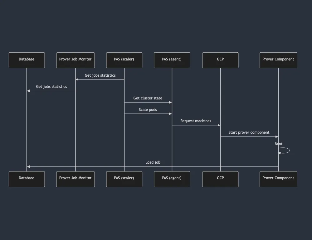
Job data is available at PJM level. PAS can connect directly to PJM to extract job information. One problem on this workflow -- different technology stack. The new PAS has been rewritten from scratch to reuse internal prover concepts. As bonus points, PAS is now open sourced (readily available for any team willing to try it out⁷).

2. Replace Keda

Keda scaling is based off metrics. A direct call model would be suitable. Keda can be replaced with an agent that receives requests to scale-up/scale-down via REST API (the agent wraps the K8s API behind the hood). Removing Keda from the workflow removes unneeded latency, simplifies setup & increases reliability.

With these changes in place, the autoscaler will have 2 components:

• scaler -- responsible for querying data from PJM, keeping state on clusters and issuing commands to agents
• agent -- aware of it's own cluster semantics and subordinate to scaler

Note 1: There is one agent per cluster, but a scaler may be connected to multiple clusters (& agents) at any given time.

Note 2: Existing autoscaling options focus on a single cluster. PAS implementation assumes multiple clusters with no guarantee that the requested hardware will be provided.

Results

AutoScaling becomes:

Previous architecture could do scaling checks at ~15 min mark. Current setup has arbitrary sensibility. In practice, this means that machines could be turned off as soon as they are needed, instead of 15 minutes after no jobs are available (worst case scenario).

With faster reaction times, the autoscaler can also have long-running components. These run continuously knowing that they will be shut down as soon as there are no other jobs to be executed. Previously, to reduce amount of idleness (15 minutes delay is a lot of lost compute), a machine was spun up to execute one job. Once it finished, the machine would terminate (known as one-off running).

Future Improvements

This implementation is v1. As it is being ran in production, more areas of improvement will show up. Of the already known:

• just-in-time scheduling; machines could be booted ahead of time, given the DAG & known execution times for each component
• communication between PAS scaler & agent can be done with lighter network usage (think gRPC)
• there is space for further optimizations on the number of jobs configuration for each component

Conclusion

All 3 aspects⁸ of proving need to cooperate in order to get fast & cheap proving. Above is a summary of changes done that are available today in main net.

The system is pending further optimizations, but expect to see a continuation of the same pattern: optimize the underlying cryptographic primitives, improve scheduling logic on top of it and match it to fastest, cost efficient hardware possible.

Sadly, there aren't graphs from the start of the optimization process to the end, but there is some data from midway to the final release. Proof of cost graph⁹¹⁰¹¹:

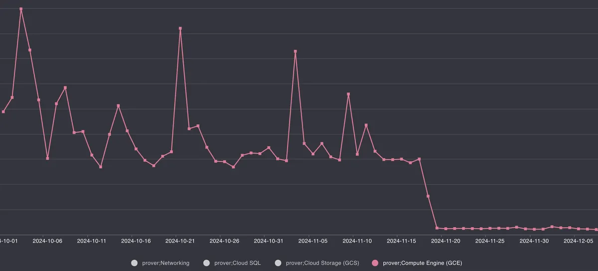^ Low TPS chain

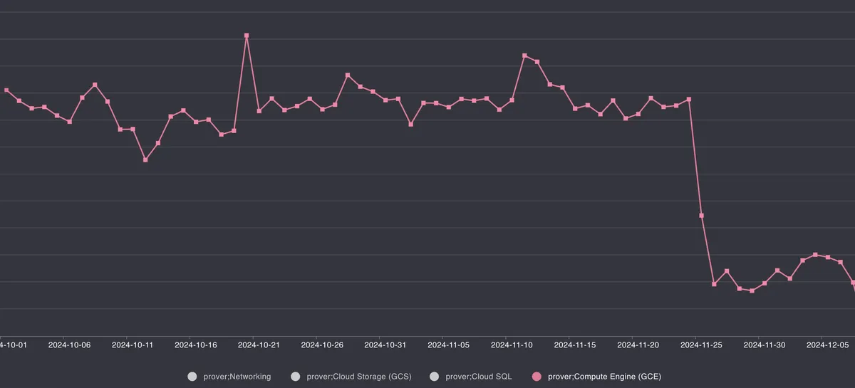^ High TPS chain